Statistical Significance for Humans — Automated Statistical Significance Calculator for A/B Testing

As online marketing grows more complex, it’s difficult to get all the details right on the first try. With dozens of decisions to make for each ad, it is no surprise that there’s often room for improvement. Fortunately there’s a way to consistently make better decisions: A/B testing.

However, running randomized controlled trials typically requires a good understanding of statistics, and most of our customers are not statisticians. We saw a clear need for a more understandable, automated solution especially for statistical significance calculations—so that’s what we set out to build.

Facebook’s Marketing API offers good tools for settings up A/B tests for Facebook ads. When building our UI for testing we wanted to make sure that the conclusions from each test are as easy as possible to understand correctly, and as difficult as possible to understand incorrectly. One big challenge was to make statistical significance understandable for non-statisticians.

The most common method of estimating statistical significance is to calculate p-values. However, considering how often p-values are misunderstood even among scientists, this isn’t exactly a user-friendly solution. And let’s face it: nobody really wants to know the p-value anyway. Or when was the last time your heard somebody ask: “Hey did you finish that A/B test? I really want to know the probability of observing data that is at least as extreme as the data we got, assuming there is no difference.”

The fundamental problem with the p-value is that it’s a very unintuitive concept and therefore far too easy to understand incorrectly. What most people really want to know is something much simpler: How likely is it that A is better than B? How much better?

But before answering those questions, let’s see what else can go wrong in statistical testing. 

Checking the outcome can change the result

In practice, calculating statistical significance after data has been collected isn’t quite enough. Our users also want to see results while the test is running, so they can end the test when enough data has been collected. This sounds reasonable enough: why spend more time and money on a test when you already know the result. This practice is known as optional stopping.

However, there’s a catch. Unless you’re very careful with the details, checking the results and stopping prematurely can alter the outcome of the test itself. This might sound surprising, but the reason is quite simple: the calculated p-value fluctuates as data is collected.

For example, suppose we decide to run a test until 1000 samples are collected, and use a significance level of 5%. This means, by definition, that assuming there is no difference you have a 5% probability of getting a false positive result. But this is true only if you evaluate the outcome exactly once at the end of the test. The p-value can dip below the 5% threshold at some point during the test, even if it’s above the threshold at the end. This means that the more often you check the more likely you’re to catch the test at a moment when the p-value is small, making the actual false positive rate larger than intended. Check too often, and the problem becomes too large to ignore.

This problem with optional stopping is similar to the multiple comparisons problem, but there are important differences. First, we don’t know in advance how many tests will be run; second, the outcomes of consecutive tests are highly correlated. Because of these differences the methods used to solve the multiple comparisons problem do not readily work in this case, which is why we decided to take a Bayesian approach.

Solving the optional stopping problem with Bayesian statistics

Bayesian statistics is the natural solution for answering questions like “How likely it is that A is better than B”. Another benefit of the Bayesian approach is that it gives us the flexibility to step around the problem described above.

The insight to solve the optional stopping problem came from a blog post by John K. Kruschke. The main idea is that if the decision to stop depends on the outcome—whether a difference exists, or how large the difference is—the test result will be affected by checking. However, if the decision to stop depends on how precisely the difference is known, we no longer change the outcome by stopping prematurely.

Some context is probably in order before diving into the implementation. In online advertising, we’re typically not so interested in measuring the number of clicks, but the actions the ads are trying to drive: purchases, orders, app installs, etc. These actions are known as conversion events. Performance is most often measured by cost-per-action, CPA.

Suppose we have two ad campaigns, A and B, and we’ve observed conversion counts CA and CB after spending SA and SB dollars in the campaigns. Assuming the conversions come from a Poisson process, the posterior distribution for the number of conversions is Gamma distribution with shape parameter of C+1 and rate parameter of 1 (assuming a suitable improper prior for simplicity).

Precision can be measured in many ways. We follow the example of Kruschke and define precision using the highest density interval (HDI) of the posterior distribution of CPA difference. This is pretty much all we need in order to implement a simple stopping rule in Python.

import numpy as np
import pymc3
N_samples = 100000
 
def get_CPA_samples(conversions, spend):
    return spend / np.random.gamma(conversions + 1, 1, N_samples)
 
def relative_difference(a, b):
    return 2.0 * np.true_divide(b - a, b + a)
 
def get_HDI(A, B, HDI_volume):
    CPA_samples_A = get_CPA_samples(A['conversions'], A['spent'])
    CPA_samples_B = get_CPA_samples(B['conversions'], B['spent'])
    diff_samples = relative_difference(CPA_samples_A, CPA_samples_B)
    return pymc3.stats.hpd(diff_samples, 1 - HDI_volume)

def evaluate_HDI(HDI, precision):
    if np.diff(HDI) > 2 * precision:
        return 'Continue testing'
    else:
        if np.prod(HDI) > 0:
            better, worse = ("A", "B") if HDI[0] > 0 else ("B", "A")
            return 'Stop the test: {} is better than {}'.format(better, worse)
        else:
            return 'Stop the test: No difference found'
        
def evaluate_data(A, B, parameters):
    HDI = get_HDI(A, B, parameters["HDI_volume"])
    return evaluate_HDI(HDI, parameters['precision'])


To calculate the recommendation for observed data we’d then use: 

parameters = {    
    "HDI_volume": 0.95,
    "precision": 0.1
}

A = {"conversions": 315, "spent": 4500}
B = {"conversions": 470, "spent": 6000}

print(evaluate_data(A, B, parameters)) 

To calculate the recommendation for observed data we’d then use: 

parameters = {        "HDI_volume": 0.95,    "precision": 0.1}A = {"conversions": 315, "spent": 4500}B = {"conversions": 470, "spent": 6000}print(evaluate_data(A, B, parameters))

If you run this code the last line should print “Continue testing”. Visualizing the posterior distributions for CPA (left) and the difference (right) shows what is going on.

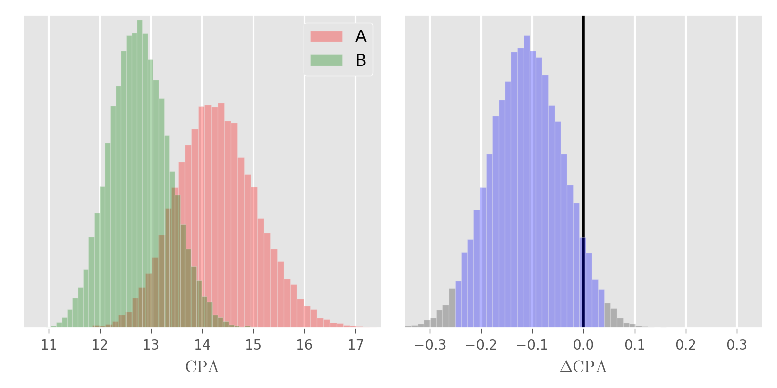
The blue area in the difference distribution represents the 95% HDI. Because its width (≈ 0.26) is larger than two times precision, the recommendation is to continue the test and collect more data.

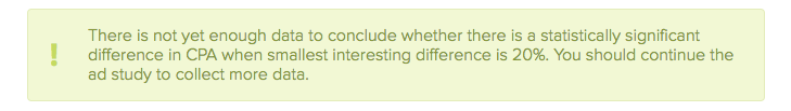
If you change precision to 15% the outcome changes to “Stop the test: No difference found”. In this case we do know the posterior with required precision, but because HDI includes zero the result is that there is no statistically significant difference.

The actual stopping rule we use has been modified to fit our use case. For example, we recommend stopping also when it’s very clear that there’s a difference even if the precision condition hasn’t been met. While this does compromise the statistical integrity of the test, in practice it’s more important to not waste money on a test whose conclusion is already clear than to get a completely rigorous estimate of the magnitude of the difference.

Also, in this example the same HDI volume—95%—is used both to decide whether to stop and to estimate whether a difference exists, which fixes both the false positive rate and the false negative rate. By using different volumes it is possible to create a stopping condition to achieve any false negative rate, at least to a good approximation.

Making precision easier to understand

Implementing the stopping rule so that it’s usable in practice took a few tries. Initially we asked users to provide the value of precision directly, but this turned out to be too difficult: in order to give a reasonable value you must understand what precision is, and to understand what precision is you need to understand all the implementation details discussed above.

So instead of precision we now ask users to provide the smallest interesting difference. This concept is meaningful in itself and therefore easier for users to define—especially when combined with automatic data requirement estimation, as will be discussed in the next chapter. We then set precision to be half of the smallest interesting difference.

Facilitating test design with power analysis

Being able to calculate statistical significance during the test is good, but even that isn’t quite enough. Decisions about schedule and budget are made already when planning the test, and thus our users need to be able to estimate how much data is needed, how much it costs to collect the data, and how long the test is likely to take. Fortunately these estimates are relatively easy to calculate using power analysis.

The most important factor for estimating data requirement is the smallest interesting difference: the smaller difference you want to find, the more data you need. In practice, however, seeing the estimate influences the value of the smallest interesting difference itself. If testing was free, you’d of course want to know every tiny difference that might exist. Only after seeing the costs can you decide what differences are worth pursuing.

By implementing the inputs as a sliders we encourage users to experiment with different values and see how that affects the total cost of the test. Pull the slider to the left and you will find that in order to detect a 5% difference in CPA you need to collect over 12,000 conversions. With a CPA of $50, that means investing $600,000 to potentially improve performance by 5%. There are probably better ways to invest that money.

Playing with the sliders can be an eye-opening experience for test designers. The fact that detecting small differences requires large amounts of data isn’t always obvious for people without statistical training, and in our experience most people tend to underestimate how much random variation there is. Before the estimation tool was available it was common to see tests stopped after collecting only 100 conversions. Such tests are all but guaranteed to be inconclusive.

Spell it out

The last step was to write out results in plain English instead of the cryptic language so often used in statistical hypothesis testing. First, the stopping rule allows us to provide instructions on what the user should do while the test is running.

When the stopping criterion is met and a difference is identified, we tell which alternative is the best one and also write out information about effect size.

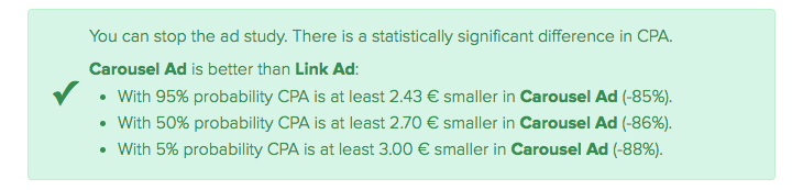
Reporting effect sizes is often overlooked even though this information is obviously valuable for the user. While we could get away with reporting only MAP estimates, this would fail to communicate the uncertainty which can be significant in some cases. Instead, we summarize the posterior of the difference distribution with three sentences. The posterior could also be visualized, but this would require users to be comfortable reading distribution plots.

When the stopping condition is met but there is no statistically significant difference, we report this to the user to avoid spending time and money chasing small differences. We also report the maximum difference that could exist based on the posterior difference distribution.

Overall, the automated statistical significance calculator has been well received by our customers. It replaces several error-prone manual steps in runnings A/B tests: gathering data, copying values to calculator tools, and interpreting results. Automating these steps allows users to focus on more important tasks—like deciding what to test next.

Interested in data science and want to learn more about Smartly? Do not miss the excellent blog post by my colleague Markus on How We Productized Bayesian Revenue Estimation with Stan.

Interested in data science, coding and crafting the best possible UX? Check out our open engineering positions and apply! www.smartly.io/developer

‍